In an earlier post, we looked at the problem and challenges of text summarization. We dove into an intuitive state-of-the-art deep learning solution and generated some sample results. The solution we presented was a sequence-to-sequence algorithm that read text inputs and learned to generate text outputs using recurrent neural networks. This class of algorithms is powerful and broadly applicable to other natural language problems such as machine translation or chatbots.
In this post, we’ll look at the practical steps needed to train a seq-to-seq model to summarize news articles. Beyond the training setup and code implementation, we’ll also look at some ideas to train the model much more quickly (decreasing time from three days to under half a day). When we’re through, we’ll be able to generate summaries like the following:
Waymo files for an injunction against Uber’s use of its self-driving tech
Waymo has taken the next step in its suit against Uber. It alleges that Otto founder Anthony Levandowski took the information while employed at Waymo when it was still Google’s self-driving car project. The suit is based on a very serious charge of intellectual property theft.
North Korea vows ‘thousands-fold’ revenge on US over sanctions
North Korea has vowed to exact “thousands-fold” revenge against the US. UN security council backed new sanctions on Saturday that could slash the regime’s $3bn in annual export revenue by a third. The measures target key revenue earners such as coal, iron, lead and seafood but not oil. The US secretary of state, Rex Tillerson, said on Monday that North Korea should halt missile launches if it wanted to negotiate.
As these seq-to-seq models and associated libraries are relatively new, we hope that sharing our learnings will make it easier to get started with research in this area.
Getting started
Deep learning framework
We’ll first need to choose a library for building our model. With the recent growth of deep learning, we have a number of good ones to choose from, most notably TensorFlow, Caffe, Theano, Keras, and Torch. Each of these supports seq-to-seq models, but we will choose to use TensorFlow here due to its
- Size of community and adoption
- Flexibility in expressing custom mathematical relationships
- Ease-of-use with good feature support (GPU, training visualization, checkpointing)
- Seq-to-seq code examples
Unfortunately, TensorFlow is also actively changing, not always fully documented, and can have a steeper learning curve, so other options could be appealing if these are important factors.
If you’re new to TensorFlow, check out the main guides. The rest of this post will use code examples, but the high-level concepts and insights can be understood without prior knowledge.
Hardware
GPU computing is really critical for speeding up training of deep learning models (sometimes on the order of 10X faster than CPUs). We can use GPUs either through a cloud-based solution like AWS or FloydHub, or by using own GPU computer; while cloud options are no longer considered cheap or even fast, they’re quick to set up. Spinning up a p2.xlarge instance on AWS with a deep learning AMI takes minutes, and TensorFlow will come installed and able to use the GPU.
Data
The next step is to get a data set to train on. The CNN / Daily Mail Q&A dataset is the most commonly used in recent summarization papers; it contains 300,000 news articles from CNN and Daily Mail published between 2007 and 2015, along with human-generated summaries of each article. The articles cover a broad range of common news topics and are on average 800 tokens (words and punctuation characters) long. The summaries are on average 60 tokens (or 3.8 sentences) long. Another data set of similar scale is the New York Times Annotated Corpus, although that has stricter licensing requirements.
We can download the data and use a library such as spaCy to prepare the dataset, in particular to tokenize the articles and summaries. Here’s a sample summary we found:
Media reports say the NSA tapped the phones of about 35 world leaders. Key questions have emerged about what Obama knew, and his response. Leaders in Europe and Latin America demand answers, say they’re outraged.
Implementing a seq-to-seq model
We’ll demonstrate how to write some key parts of a seq-to-seq model with attention, augmented with the pointer-copier mechanism See et al., 2017. (Check out our earlier post for an overview of the model). The model is approximately the state-of-the-art, in terms of the standard ROUGE metric for summarization. (Note: this metric is fairly naive, as it does not give credit to summaries that use words or phrases that aren’t in the gold-standard summary, and it does not necessarily penalize summaries that are grammatically incorrect).
Batched inputs
The input data that we feed to our model during training are going to be the sequence of tokens in an article and its corresponding summary. Although we start off with token strings, we will want to pass in token IDs to the model. To do this, we define a mapping from the 50K most common token strings in the training data to a unique token ID (and a special “unknown” token ID for the remaining token strings).
During training, we want to feed in a batch of examples at once, so that the model can make parameter updates using stochastic gradient descent. We thus define the placeholders to be 2D tensors of token IDs, where rows represent individual examples and columns represent time steps.
# The token IDs of the article, to be fed to the encoder.
article_tokens = tf.placeholder(dtype=tf.int32, shape=[batch_size, max_encoder_steps])
# The number of valid tokens (up to max_encoder_steps) in each article.
article_token_lengths = tf.placeholder(dtype=tf.int32, shape=[batch_size])

# The token IDs of the summary, to be fed to the decoder and used as target outputs.
summary_tokens = tf.placeholder(dtype=tf.int32, shape=[batch_size, max_decoder_steps])
# The number of valid tokens (up to max_decoder_steps) in each summary.
summary_token_lengths = tf.placeholder(dtype=tf.int32, shape=[batch_size])
Note that our sequentially-valued placeholders accept fixed-size tensors, where the length of the tensors in the sequence dimension are chosen hyperparameters (max_encoder_steps , max_decoder_steps). For sequences that are shorter than these dimensions, we pad the sequence with a special padding token.
Defining the model graph
Here’s a start to defining the TensorFlow graph, which transforms the input batch of article tokens to the output word distributions at each time step.
# Embedding
embedding_layer = tf.get_variable(
    name='embedding',
    shape=[vocab_size, embedding_dim],
    dtype=tf.float32,
)
encoder_inputs = tf.nn.embedding_lookup(embedding_layer, article_tokens)
decoder_inputs = tf.nn.embedding_lookup(embedding_layer, summary_tokens)

# Encoder
forward_cell = tf.nn.rnn.LSTMCell(encoder_hidden_dim)
backward_cell = tf.nn.rnn.LSTMCell(encoder_hidden_dim)
encoder_outputs, final_forward_state, final_backward_state = (
    tf.nn.bidirectional_dynamic_rnn(
        forward_cell,
        backward_cell,
        encoder_inputs,
        # Tells the method how many valid tokens each input has, so that it will
        # ignore the padding tokens. article_token_lengths has shape [batch_size].
        sequence_length=article_token_lengths,
    )
)

# Decoder with attention
...

# Compute output word distribution
...
The embedding layer allows us to map each token ID to a vector representation (or word embedding). The token embeddings are fed to our bi-directional LSTM encoder, using the high-level method tf.nn.bidirectional_dynamic_rnn().
There’s some more work needed to complete the model definition; the code from See’s paper is on GitHub, as is this more concise example.
Training operation
One common loss function for seq-to-seq models is the average log probability of producing each target summary token. To get our training operation, we need to compute the gradients of the loss. When dealing with sequential models, it’s possible that the gradients can “explode” in size, since they get multiplied at each time step through backpropagation. To account for this, we “clip” or reduce the gradient magnitude to some maximum norm. These clipped gradients can be used to update the variables using an optimization algorithm (we choose Adam here).
    # Define loss
    loss = tf.reduce_mean(target_log_probs)
    tf.summary.scalar('loss', loss) # save loss for logging

    # Compute gradients
    training_vars = tf.trainable_variables()
    gradients = tf.gradients(loss, training_vars)
    # Clip gradients to a maximum norm
    gradients, global_norm = tf.clip_by_global_norm(gradients, max_grad_norm)
    # Apply gradient update using Adam
    optimizer = tf.train.AdamOptimizer()
    train_op = optimizer.apply_gradients(zip(gradients, training_vars))
Training loop
After defining the model, we run training steps to learn good parameter values, by passing in batched inputs and asking the model to run the training operation. There are challenges with running long training jobs; using the Supervisor class here helps us in two ways:
- Saves checkpoints of the model during training, so that we can stop and restart jobs
- Saves summary values like loss to help visualize progress of training
sv = tf.train.Supervisor(saver=tf.train.Saver(), **kwargs)
with sv.prepareorwaitforsession() as sess:
while True:
batchdict = batcher.nextbatch()# Run training step and fetch some training info _, summaries_value = sess.run( fetches=( train_op, # 'summaries' is a string from the tf.summary module that saves # specified fields during training. Useful for visualization. summaries, ), feed_dict=batch_dict, ) # Writes summary info that can be viewed through TensorBoard UI. sv.summary_writer.add_summary(summaries_value)
Hyperparameters
Here are some sensible values for key hyperparameters, based on See’s paper and other recent literature.
vocab_size = 50000
embedding_dim = 128
encoder_hidden_dim = 250
decoder_hidden_dim = 400
batch_size = 16
max_encoder_steps = 400
max_decoder_steps = 100
Training speed
With our model now defined, we’re ready to train it. Unfortunately, deep learning methods typically take a long time to train, due to the size of the data and the large number of model parameters.
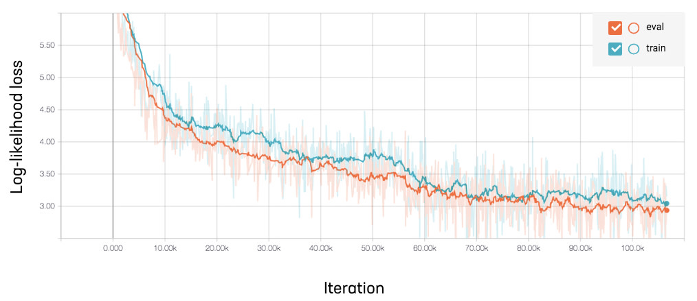
As See notes in her paper, we can begin training on shorter inputs and labels. While the algorithm will ultimately use the first 400 tokens of each article and the first 100 tokens of each summary for training, the initial training steps do not need to utilize all of that information. By starting off with smaller examples (e.g. 150 token articles and 75 token summaries), we can run iterations that take less time, leading to overall faster convergence.
Here’s a graph from TensorBoard of the training loss as a function of training iterations. Note that we increased article token size from 150 to 400 at around iteration 55K, when the loss started to flatten out. The change noticeably decreases the loss, but also decreases speed from .85 to .6 training steps per second. In total, the training took nearly two days with around 6 epochs (See states that fully training the model took 3 days).

Progress of training loss

Speed of each training iteration
The long training cycle is not only an inconvenience; training time is a huge bottleneck for experimenting with new ideas as well as uncovering bugs, which in turn is a bottleneck for making research progress.
We’ve discovered some additional tricks to drastically reduce training time. The time to train a new model from scratch can be reduced under these circumstances to under half a day, with no practical decrease in summary quality. In some cases, we can even reuse trained models to initialize a new model, and then need only a few further hours for training.
Use pretrained word embeddings
Let’s take a look at where a large fraction of our model parameters are, to see if we can optimize how we use them. The word embedding layer, which maps token IDs to vectors, supplies inputs to the encoder and decoder. This size of this layer is ∗ vocabsize∗wordembeddingdim\mathsf{vocab\_size * word\_embedding\_dim}, in our case 50K∗128≈6 million50K∗128≈6 million50\text{K} * 128 \approx 6\text{ million}. Wow!
While the embedding layer can be randomly initialized, we can also use pretrained word embeddings (e.g. GloVe) as the initial embedding values. This way we begin training with a sensible representation of individual words and need fewer iterations to learn the final values.
pretrained_embedding = np.load(pretrained_embeddings_filepath)
assert pretrained_embedding.shape == (vocab_size, embedding_dim)
embedding_layer = tf.get_variable(
    name='embedding',
    shape=[vocab_size, embedding_dim],
    dtype=tf.float32,
    inital_value=pretrained_embedding,
)
Reduce vocab size
To simplify the embedding layer even further, we can reduce the vocab size. Looking at the tail end of our original 50K word vocabulary, we find words like “landscaper” and “lovefilm”, which appear in the training set less than a hundred times. It’s probably difficult to learn much about these words when the label for each article is a summary that may or may not utilize these words, so we should be able to reduce the vocab size without incurring much loss of performance. Indeed, reducing vocab size to 20K seems fine, especially if we replace the out-of-vocab words with a token corresponding to its part-of-speech.
Use tied output projection weights
The other large component of the total trainable parameters is in the output projection matrix WprojWprojW_{proj}, which maps the decoder’s hidden state vector (dimension hhh) to a distribution over the output words (dimension vvv).

Using the projection matrix to map hidden state to output distribution
The number of parameters in WprojWprojW_{proj} is v⋅h=50K∗400≈20 million(!!)v⋅h=50K∗400≈20 million(!!)v \cdot h = 50\text{K} * 400 \approx 20\text{ million}(!!)in our case. To reduce this number, we can instead express the matrix as

Factorization of the projection matrix
where WembWembW{emb} is the word embedding matrix with embedding size eee. By restricting the projection matrix to be of this form, we reuse syntactic and semantic information about each token from the embedding matrix and reduce the number of new parameters in WsmallprojWsmallprojW{small\_proj} to e⋅h=128∗400≈50Ke⋅h=128∗400≈50Ke \cdot h = 128 * 400 \approx 50\text{K}.
w_small_proj = tf.get_variable(
    name='w_small_proj',
    shape=[embedding_dim, decoder_hidden_dim],
    dtype=tf.float32,
)
# shape [decoder_hidden_dim, vocab_size]
w_proj = tf.matmul(embedding, w_small_proj)
b_proj = tf.get_variable(name='b_proj', shape=[vocab_size], dtype=tf.float32)

# shape [vocab_size]
output_prob_dist = w_proj * decoder_output + v
Cumulative impact on training time
Using these tricks (and a few more), we can compare the training of the original and new versions side by side. In the new version, during training we again increase the token size of the training articles from 150 to 400, this time at iteration 8000. Now we reach similar loss scores in under 20K iterations (just over one epoch!), and in total time of around 6 hours.

Comparison of training progress between original and improved versions
Reusing previously trained models
At times, we can also reuse a previously trained model instead of retraining one from scratch. If we are experimenting with certain model modifications, we can initialize the values of the variables to those from earlier iterations. Examples of such modifications include adding a loss to encourage the model to be more abstractive, adding additional variables to utilize previous attention values, or changing the training process to use scheduled sampling. This can save us a ton of time by jumping straight to a trained model instead of starting from randomly initialized parameters.
We can reload previous variables with the below idea, assuming we have kept the variable names consistent from model to model.
# Define the placeholders, variables, model graph, and training op
model.build_graph()

# Initialize all parameters of the new model
sess = tf.Session()
sess.run(tf.global_variables_initializer())

# Initialize reusable parameter values from the old model
saver = tf.train.Saver([v for v in tf.global_variables() if is_reusable_variable(v)])
saver.restore(sess, old_model_checkpoint_path)
Evaluation speed
How long does our model take to summarize one article? For deployment, this becomes the key question instead of training time. When generating summaries, we encode 400 article tokens, and decode up to 100 output tokens with a beam search of size 4. Running it on a few different hardware configurations, we find:
| Hardware | Time per summary | |||
|---|---|---|---|---|
| CPU* (single core) | 17.2s | |||
| CPU* (4 cores) | 8.1s | |||
| GPU | 1.5s |
* TensorFlow not compiled from source (which may increase runtimes by 50%)
Unsurprisingly, the GPU really helps! On the other hand, needing to run the algorithm at scale using CPUs looks like a very challenging task.
Looking more closely, we see that with one CPU, running the encoder takes about .32 seconds and running each decoding step (which, in beam search, extends each of beamsize_ partial summaries by one token) takes about .18 seconds. (The rest of the time not spent inside a TensorFlow session is less than a second). Looking even further at the trace of one decoding step, we find:

Timing breakdown of a decoder step. Note: in this analysis, we have already precomputed the product for the W_proj matrix, so that it is not recomputed at every step.
Interestingly, nearly all of the steps before the final “MatMul” involve computations for the attention distribution over the article words. As the vast majority of the original 17 seconds are spent doing numerical computations, we might need to resort to hardware upgrades of using GPU / more CPUs / compiling TensorFlow from source in order to significantly improve performance.
Reflections
Having iterated over and analyzed these models, here are some of our thoughts on the state of developing seq-to-seq models today.
First, despite our efforts (or perhaps as justification for our efforts), the time needed to evaluate new ideas is quite long. We tried to speed up training by reducing the size and dimensions of our models and datasets, but that only goes so far. Scaling up the number of computers for a training task can be difficult for both mathematical and engineering reasons. Additionally, to evaluate a new version of the model, we had to manually inspect the results against a common set of evaluation articles, since we did not have a good metric for summarization. One consequence of slow iteration cycles is that there isn’t much flexibility to do extensive hyperparameter searches. It’s great when we can use the literature to guide our choices here.
Testing out new ideas is made even harder by how challenging it is to correctly implement them. Many deep learning concepts are newly added, updated, or deprecated in TensorFlow, resulting in incomplete documentation. It’s very easy to make implementation mistakes with subtle side effects; some errors don’t trigger exceptions, but instead compute values incorrectly and are only discovered when training doesn’t converge properly. We found it useful to manually check inputs, intermediate values, and outputs for most changes we made. In managing our code, we found it important to create flags for every new model variant and keep each commit compatible with older running experiments.
We were impressed that the deep learning model could train so easily. Given just one possible summary for each article, the model could learn millions of parameter weights, randomly initialized, from the embeddings to the encoder to the decoder to attention to learning when to copy. We’re excited to continue to work with seq-to-seq models as state-of-the-art solutions to NLP problems, especially as we improve our understanding of them.
Reference
Abigail See, Peter J. Liu, and Christopher D. Manning. 2017. “Get to the Point: Summarization with Pointer-Generator Networks.” CoRR abs/1704.04368. http://arxiv.org/abs/1704.04368.